Module 6 Answer Key
6.11 Exercises
A. Problem: Project Evaluation Methods at Topley
1. Payback period
[latex]\frac{{220,000}}{{50,000}}[/latex] = 4.4 years
2. Discounted payback period
| Year | Cash Flow | Discount Factor | Present Value | Cumulative Present Value |
| 0 |
-220,000 |
(1 .16)^0 |
-220,000.00 |
-220,000.00 |
| 1 |
50,000 |
(1 .16)^1 |
43,103.45 |
-176,896.55 |
| 2 |
50,000 |
(1 .16)^2 |
37,158.15 |
-139,738.40 |
| 3 |
50,000 |
(1 .16)^3 |
32,032.88 |
-107,705.52 |
| 4 |
50,000 |
(1 .16)^4 |
27,614.55 |
-80,090.97 |
| 5 |
50,000 |
(1 .16)^5 |
23,805.65 |
-56,285.32 |
| 6 |
50,000 |
(1 .16)^6 |
20,522.11 |
-35,763.21 |
| 7 |
50,000 |
(1 .16)^7 |
17,691.48 |
-18,071.73 |
| 8 |
50,000 |
(1 .16)^8 |
15,251.27 |
-2,820.46 |
| 9 |
50,000 |
(1 .16)^9 |
13,147.65 |
10,327.19 |
| 10 |
50,000 |
(1 .16)^10 |
11,334.18 |
21,661.37 |
Discounted payback period = 8 + [latex]\frac{{2,820.46}}{{13,147.65}}[/latex] = 8.21 years
3. NPV
50,000 [latex](\frac{{1 - {{\left( {1 + .16} \right)}^{ - 10}}}}{{.16}}[/latex]) = 241,661.37
241,661.37 – 220,000 = 21,661.37
NPV is what remains after compensating investors for the RRR of 16%. This is the excess profit of the project in dollar terms and is equivalent to 2.60% in Part 4.
4. IRR
220,000 = 50,000 [latex](\frac{{1 - {{\left( {1 + i} \right)}^{ - 10}}}}{i}[/latex])
i = .1860 or 18.60%
The RRR of the project is 16.00%, so the project is earning 2.60% more than required. This is the excess profit of the project in per cent terms.
Note: The IRR function in Excel can be used to solve for i.
5. Modified IRR
| Year | Cash Flow | FV Factor | FV (16.0%) | FV (18.6%) |
| 1 |
50,000 |
(1 i)9 |
190,148.07 |
232,130.50 |
| 2 |
50,000 |
(1 i)8 |
163,920.75 |
195,725.55 |
| 3 |
50,000 |
(1 i)7 |
141,310.99 |
165,029.97 |
| 4 |
50,000 |
(1 i)6 |
121,819.82 |
139,148.38 |
| 5 |
50,000 |
(1 i)5 |
105,017.09 |
117,325.78 |
| 6 |
50,000 |
(1 i)4 |
90,531.97 |
98,925.62 |
| 7 |
50,000 |
(1 i)3 |
78,044.80 |
83,411.15 |
| 8 |
50,000 |
(1 i)2 |
67,280.00 |
70,329.80 |
| 9 |
50,000 |
(1 i)1 |
58,000.00 |
59,300.00 |
| 10 |
50,000 |
(1 i)0 |
50,000.00 |
50,000.00 |
|
1 1,066,073.50 |
2 1,211,326.80 |
[latex]\begin{array}{l}{}^1\;220,000 = \frac{{1,066,073.50}}{{{{\left( {1 + i} \right)}^{10}}}}\quad \quad i = .1709\quad \\{}^2\;220,000 = \frac{{1,211,326.80}}{{{{\left( {1 + i} \right)}^{10}}}}\quad \quad i = .1860\quad \end{array}[/latex]
MIRR is 17.09%
6. PI
[latex]{\rm{\;}}\frac{{241,661.37}}{{220,000}}[/latex] = 1.10
B. Problem: Project Evaluation Methods at Cott Beverages
- Payback period
Year Cumulative Cash Flows 1 10,000
2 18,000
3 24,000
4 29,000
5 33,000
6 36,000
7 39,000
3 + [latex](\frac{{28,000 - 24,000}}{{\begin{array}{*{20}{c}}{29,000 - 24,000}\\{}\end{array}}}[/latex]) (1) = 3.8 years
- Discounted payback period
Year Cash Flow Discount Factor Present Value Cumulative Present Value 0 (28,000)
(1 .16)^0
-28,000.00
-28,000.00
1 10,000
(1 .16)^1
8,620.69
-19,379.31
2 8,000
(1 .16)^2
5,945.30
-13,434.01
3 6,000
(1 .16)^3
3,843.95
-9,590.06
4 5,000
(1 .16)^4
2,761.46
-6,828.60
5 4,000
(1 .16)^5
1,904.45
-4,924.15
6 3,000
(1 .16)^6
1,231.33
-3,692.82
7 3,000
(1 .16)^7
1,061.49
-2,631.33
Project does not break even on a present value basis.
- NPV
Year Cash Flow Discount Factor Present Value 1 10,000
(1 .16)^1
8,620.69
2 8,000
(1 .16)^2
5,945.30
3 6,000
(1 .16)^3
3,843.95
4 5,000
(1 .16)^4
2,761.46
5 4,000
(1 .16)^5
1,904.45
6 3,000
(1 .16)^6
1,231.33
7 3,000
(1 .16)^7
1,061.49
Total 25,368.67
25,368.67 – 28,000.00 = <2,631.33>
The project is not earning its RRR of 16% as the NPV is negative.
- IRR
28,000 = [latex](\frac{{10,000}}{{{{\left( {1 + i} \right)}^1}}}[/latex]) + [latex](\frac{{8,000}}{{{{\left( {1 + i} \right)}^2}}}[/latex]) + [latex](\frac{{6,000}}{{{{\left( {1 + i} \right)}^3}}}[/latex]) + [latex](\frac{{5,000}}{{{{\left( {1 + i} \right)}^4}}}[/latex]) + [latex](\frac{{4,000}}{{{{\left( {1 + i} \right)}^5}}}[/latex]) + [latex](\frac{{3,000}}{{{{\left( {1 + i} \right)}^6}}}[/latex]) + [latex](\frac{{3,000}}{{{{\left( {1 + i} \right)}^7}}}[/latex])
i = .1186 or 11.86%
Project is not earning the RRR of 16%.
Note: IRR function in Excel can be used to solve for i.
5. PI
[latex]\frac{{25,368.67}}{{28,000.00}}[/latex] = .91
C. Problem: Standalone Decision at Rogers
- No
Initial investment -120,000.00
Tax Shield (120,000) (.45) [latex](\frac{{.25}}{{.25 + .12}}[/latex]) [latex](\frac{{2 + .12}}{{2\left( {1 + .12} \right)}}[/latex]) 34,531.85
Increase in working capital -5,000.00
1Annual savings 71,332.15
Salvage value (10,000) / (1 .12)4 6,355.18
Lost tax shield (10,000) (.45) [latex](\frac{{.25}}{{.25 + .12}}[/latex]) [latex](\frac{{2 + .12}}{{2\left( {1 + .12} \right)}}[/latex]) / (1+.12)4 -1,828.80
Decrease in working capital (5,000) / (1 .12)4 3,177.59
NPV
-11,432.03
190,000 – 22,000 – 6,000 – 3,300 – 7,000 – 9,000 = 42,700
(42,700) (1 – .45) [latex](\frac{{1 - {{\left( {1 + .12} \right)}^{ - 4}}}}{{.12}}[/latex]) = 71,332.15
- Yes
(200) (90,000/450) – (22,000) – (200) (6,000/450) – (200) (7,000/450) – (200) (9,000/450) = 8,222.22
(8,222.22) (1 – .45) [latex](\frac{{1 - {{\left( {1 + .12} \right)}^{ - 4}}}}{{.12}}[/latex]) = 13,735.57
-11,432.03 + 13,735.57 = 2,303.54
D. Problem: Replacement Decision at Ruby
- Yes
Net investment (500,000 – 50,000) -450,000.00
Tax shield (450,000) (.35) [latex](\frac{{.2}}{{.2 + .10}}[/latex]) [latex](\frac{{2 + .10}}{{2\left( {1 + .10} \right)}}[/latex]) 100,277.27
Increase in net working capital -10,000.00
Annual saving (200,000) (2) (1-.35) [latex](\frac{{1 - {{\left( {1 + .10} \right)}^{ - 8}}}}{{.10}}[/latex]) + (20,000) (4 + 2) (1-.35)) [latex](\frac{{1 - {{\left( {1 + .10} \right)}^{ - 8}}}}{{.10}}[/latex])
1,803,205.05
Salvage value (80,000-10,000) / (1 .10)8 32,655.52
Lost tax shield (80,000-10,000) (.35) [latex](\frac{{.2}}{{.2 + .10}}[/latex]) [latex](\frac{{2 + .10}}{{2\left( {1 + .10} \right)}}[/latex]) / (1+.10)8 -7,273.27
Decrease in net working capital (10,000) / (1 .10)8 4,655.07
NPV
1,473,469.64
E. Problem: Replacement Decision at Zebra
- Yes
Net investment (141,000 – 10,000) -131,000.00
Tax shield (131,000) (.31) [latex](\frac{{.2}}{{.2 + .115}}[/latex]) [latex](\frac{{2 + .115}}{{2\left( {1 + .115} \right)}}[/latex]) 24,454.45
Decrease in net working capital 30,000.00
1 Annual savings (191,250) (1-.31) [latex](\frac{{1 - {{\left( {1 + .115} \right)}^{ - 6}}}}{{.115}}[/latex]) 550,322.43
Salvage value (18,000) / (1 .115)6 9,367.49
Lost tax shield (18,000) (.31) [latex](\frac{{.2}}{{.2 + .115}}[/latex]) [latex](\frac{{2 + .115}}{{2\left( {1 + .115} \right)}}[/latex]) / (1+.115)6 -1,748.68
Increase in net working capital (30,000) / (1+.115)6 -15,612.49
NPV 465,783.20
1
Additional units (12.00-5.75) (15,000) 93,750 Savings – VC (7.50-5.75) (50,000) 87,500 Savings – FC 10,000 Total
191,250
F. Problem: Standalone Decision with Inflation at Weatherly
- Nominal approach
Investment -3,500,000 Tax shield (3,500,000) (.21) [latex](\frac{{.3}}{{.3 + .09}}[/latex]) [latex](\frac{{2 + .09}}{{2\left( {1 + .09} \right)}}[/latex]) 542,043 1Annual savings 2,776,826 Salvage value (450,000) (1 .02)5 / (1 .09)5 322,910 Lost tax shield (496,836) (.21) [latex](\frac{{.3}}{{.3 + .09}}[/latex]) [latex](\frac{{2 + .09}}{{2\left( {1 + .09} \right)}}[/latex]) / (1 + .09)5 -50,009 NPV
91,770 1 (6,000) (16) (17.21 – 5.24) – (2) (115,000) – 65,000 = 854,120
(854,120) (1 – .21) = 674,755
Year 1 (674,755) (1 + .02)1 / (1 + .09)1 = 631,422
Year 2 (674,755) (1 + .02)2 / (1 + .09)2 = 590,872
Year 3 (674,755) (1 + .02)3 / (1 + .09)3 = 552,926
Year 4 (674,755) (1 + .02)4 / (1 + .09)4 = 517,417
Year 5 (674,755) (1 + .02)5 / (1 + .09)5 = 484,189
Total PV = 2,776,826
- Real approach
(1 + .09) = (1 + .02) (1 + Real rate)
Real rate = .0686
| Investment |
-3,500,000 |
| Tax shield (3,500,000) (.21) [latex](\frac{{.3}}{{.3 + .0686}}[/latex]) [latex](\frac{{2 + .0686}}{{2\left( {1 + .0686} \right)}}[/latex]) |
579,008 |
| 1Annual savings |
2,777,030 |
| Salvage value (450,000) / (1 .0686)5 |
322,951 |
| Lost tax shield (450,000) (.21) [latex](\frac{{.3}}{{.3 + .0686}}[/latex]) [latex](\frac{{2 + .0686}}{{2\left( {1 + .0686} \right)}}[/latex]) / (1 .0686)5 |
-53,426 |
|
NPV |
125,563 |
1 (6,000) (16) (17.21 – 5.24) – (2) (115,000) – 65,000 = 854,120
(854,120) (1 – .21) = 674,755
Year 1 (674,755) / (1 + .0686)1 = 631,438
Year 2 (674,755) / (1 + .0686)2 = 590,902
Year 3 (674,755) / (1 + .0686)3 = 552,969
Year 4 (674,755) / (1 + .0686)4 = 517,470
Year 5 (674,755) / (1 + .0686)5 = 484,251
Total PV = 2,777,030
Why are the NPVs for the nominal and real approach not equal? It is due to more than simply rounding error. Under the nominal approach, it is assumed that future cash flows will increase by 2.0% each year and that the nominal discount rate of 9.0% has an allowance for this inflation plus the real rate. Under the real approach, the increase in future cash flows due to inflation is ignored and inflation is left out of the discount rate as well and all discounting is done at the real rate of 6.86% – inflation essentially cancels out in the numerator and denominator.
When the CAD 3,000,000 is put in a CCA pool, the government does not allow these amounts to be increased each year to compensate for inflation. The government has considered indexing the contents of CCA pools but has decided against it because of the magnitude of lost tax revenues. As a result, the RRR used in the present value of CCA tax shield calculation must be 9.0% and not 6.86% since the value of the pool does not rise by the inflation rate each year. There is no inflation in the numerator to cancel out with the denominator.
The correct calculation of the NPV under the real approach is:
| Investment |
-3,500,000 |
| Tax shield (3,500,000) (.21) [latex](\frac{{.3}}{{.3 + .09}}[/latex]) [latex](\frac{{2 + .09}}{{2\left( {1 + .09} \right)}}[/latex]) |
542,043 |
| 1Annual savings |
2,777,030 |
| Salvage value (450,000) / (1 .0686)5 |
322,951 |
| Lost tax shield (450,000) (.21) [latex](\frac{{.3}}{{.3 + .09}}[/latex]) [latex](\frac{{2 + .09}}{{2\left( {1 + .09} \right)}}[/latex]) / (1 .0686)5 |
-50,015 |
|
NPV |
92,009 |
1 (6,000) (16) (17.21 – 5.24) – (2) (115,000) – 65,000 = 854,120
(854,120) (1 – .21) = 674,755
Year 1 (674,755) / (1 + .0686)1 = 631,438
Year 2 (674,755) / (1 + .0686)2 = 590,902
Year 3 (674,755) / (1 + .0686)3 = 552,969
Year 4 (674,755) / (1 + .0686)4 = 517,470
Year 5 (674,755) / (1 + .0686)5 = 484,251
Total PV = 2,776,826
3. The general inflation estimates of 2.0% is reasonable for operating costs, but not for metal prices. The price of most metals is unstable. A more thorough analysis of the metal price over the next five years is needed before a decision can be made. Even with this, the price of most metals is difficult to forecast meaning project risk is high.
G. Problem: Standalone Decision with Inflation at Quaker
- No
.05 .03 = .08
(1 + .08) = (1 .0250) (1 + X)
X = .0537
| Net investment | (2,500,000) (.95) |
-2,375,000 |
| Tax Shield | (2,375,000) (.3) [latex](\frac{{.20}}{{.20 + .08}}[/latex]) [latex](\frac{{2 + .08}}{{2\left( {1 + .08} \right)}}[/latex]) |
490,079.31 |
| Change in NWC | (2,900,000) (.3) |
-870,000 |
| 1Annual Savings |
2,241,556.23 |
|
| Change in NWC | ((3,500,000) (.3) – (2,900,000) (.3)) / (1 .0537)6 |
-131,513.59 |
| Overhaul | (850,000) (.95) / (1 .0537)6 |
-589,984.57 |
| Tax Shield | (850,000) (.95) (.3) [latex](\frac{{.20}}{{.20 + .08}}[/latex]) [latex](\frac{{2 + .08}}{{2\left( {1 + .08} \right)}}[/latex]) / (1 + .0537)6 |
121,742.85 |
| Salvage value | 350,000 / (1 .0537)12 |
186,837.60 |
| Lost Tax Shield | (350,000) (.3) [latex](\frac{{.20}}{{.20 + .08}}[/latex]) [latex](\frac{{2 + .08}}{{2\left( {1 + .08} \right)}}[/latex]) / (1 .0537)12 |
-38,553.79 |
| Change in NWC | (3,500,000) (.3) / (1 .0537)12 |
560,512.80 |
|
NPV |
-272,805.51 |
1Years 1–6
(2,900,000 – 1,900,000 – 800,000) = 200,000
(200,000) (1 – .3) [latex](\frac{{1 - {{\left( {1 + .0537} \right)}^{ - 6}}}}{{.0537}}[/latex]) = 702,265.44
Years 7–12
(3,500,000 – 2,100,000 – 800,000) = 600,000
(600,000) (1 – .3) [latex](\frac{{1 - {{\left( {1 + .0537} \right)}^{ - 6}}}}{{.0537}}[/latex]) / (1 + .0537)6 = 1,539,290.79
H. Problem: Capital Rationing at Bosie
- D and F
Project
Investment
Profitability Index
NPV
Selection
Total Investment
Total NPV
A
4,000,000
1.18
720,000
0
B
3,000,000
1.08
240,000
0
C
5,000,000
1.33
1,650,000
0
D
6,000,000
1.31
1,860,000
1
6,000,000
1,860,000
E
4,000,000
1.19
760,000
0
F
6,000,000
1.20
1,200,000
1
6,000,000
1,200,000
G
4,000,000
1.18
720,000
0
Total
12,000,000
3,060,000
See Excel spreadsheet
I. Problem: Projects of Varying Lives at Wilson
- Project 1 (Best Project)
[latex]\begin{array}{l}23,000\left( {\frac{{1 - {{\left( {1 + .07} \right)}^{ - 5}}}}{{.07}}} \right) - 55,000 = 39,304.54\\39,304.54 + \frac{{39,304.54}}{{{{\left( {1 + .07} \right)}^5}}} = 67,328.13\end{array}[/latex]
Project 2
[latex]15,000\left( {\frac{{1 - {{\left( {1 + .07} \right)}^{ - 10}}}}{{.07}}} \right) - 60,000 = 45,353.72[/latex]
- Project 1 (Best Project)
[latex]39,304.54 = {\rm{P}}\left( {\frac{{1 - {{\left( {1 + .07} \right)}^{ - 5}}}}{{.07}}} \right)\quad \quad {\rm{P}} = 9,586.01[/latex]
Project 2
[latex]45,353.72 = {\rm{P}}\left( {\frac{{1 - {{\left( {1 + .07} \right)}^{ - 10}}}}{{.07}}} \right)\quad \quad {\rm{P}} = 6,457.35[/latex]
- The assumption is that once the project is complete it can be repeated with the same return. For routine projects like machinery replacement this is reasonable, but for one-time projects like new products this is not reasonable.
J. Problem: Projects of Varying Lives at Jensen
- Project 1 (Best Project)
[latex]\frac{{40,000}}{{{{\left( {1 + .08} \right)}^1}}} + \frac{{38,000}}{{{{\left( {1 + .08} \right)}^2}}} + \frac{{42,000}}{{{{\left( {1 + .08} \right)}^3}}} - 65,000 = 37,956.87[/latex]
[latex]37,956.87 + \frac{{37,956.87}}{{{{\left( {1 + .08} \right)}^3}}} = 68,088.25[/latex]
Project 2
[latex]27,000\left( {\frac{{1 - {{\left( {1 + .08} \right)}^{ - 6}}}}{{.08}}} \right) - 79,000 = 45,817.75[/latex]
- Project 1 (Best Project)
[latex]37,956.87 = P\left( {\frac{{1 - {{\left( {1 + .08} \right)}^{ - 3}}}}{{.08}}} \right)\quad \quad P = 14,728.54[/latex]
Project 2
[latex]45,817.75 = P\left( {\frac{{1 - {{\left( {1 + .08} \right)}^{ - 6}}}}{{.08}}} \right)\quad \quad P = 9,911.08[/latex]
4. The assumption is that once the project is complete it can be repeated with the same return. For routine projects like machinery replacement this is reasonable, but for one-time projects like new products this is not reasonable.
K. Problem: Changes in Net Working Capital at Amsterdam
1.
| Year | Net Working Capital | Change in Net Working Capital |
|
2012 |
2,500,000 / 9.1 = 274,725 |
|
|
2013 |
3,400,000 / 7.9 = 430,380 |
155,655 |
|
2014 |
3,800,000 / 7.9 = 481,013 |
50,633 |
|
2015 |
3,900,000 / 7.9 = 493,671 |
12,658 |
|
12015 |
493,671 – 274,725 = 218,946 |
-218,946 |
NWC will rise over the life of the project (2013 – CAD 155,655, 2014 – CAD 50,633, 2015 – CAD 12,658) before returning to its original level (CAD 274,725) at the end of 2015.
L. Problem: Taxation Effects of Terminal Cash Flows
1.
Case 1
Terminal Cash Flows
Sale of land 4,000,000
1Capital gains tax -525,000
1(4,000,000 – 1,000,000) (.50) (.35)
What if the land is sold for CAD 500,000?
Terminal Cash Flows
Sale of land 500,000
1Capital loss benefit 87,500
1(500,000 – 1,000,000) (.50) (.35)
Case 2
Terminal Cash Flows
Sales of building 600,000
1Capital gain -17,500
2Recapture -53,804
1(600,000 – 500,000) (.5) (.35)
2(346,275 – 500,000) (.35)
What if the building is sold for CAD 100,000?
Terminal Cash Flows
Sale of building 100,000
1Terminal loss 86,196
1(346,275 – 100,000) (.35)
Case 3
Terminal Cash Flows
Sale of equipment 50,000
1Present value of future CCA 13,040
1(102,042 – 50,000) (.35) [latex](\frac{{.30}}{{.30 + .10}}[/latex]) [latex](\frac{{2 + .10}}{{2\left( {1 + .10} \right)}}[/latex])
What if the equipment is sold for CAD 120,000?
Terminal Cash Flows
Sales of equipment 120,000
1Present value of future CCA -4,500
1(102,042 – 120,000) (.35) [latex](\frac{{.30}}{{.30 + .10}}[/latex]) [latex](\frac{{2 + .10}}{{2\left( {1 + .10} \right)}}[/latex])
What if the equipment is sold for CAD 600,000?
Terminal Cash Flows
Sales of equipment 600,000
1Capital gains tax -17,500
2Present value of future CCA -97,716
1(600,000 – 500,000) (.5) (.35)
2(102,042 – 500,000) (.35) [latex](\frac{{.30}}{{.30 + .10}}[/latex]) [latex](\frac{{2 + .10}}{{2\left( {1 + .10} \right)}}[/latex])
M. Problem: Managing Risk by Adjusting the Discount Rate at Rexall
- Yes
(1 .09) = (1 Real rate) (1 .025)
Real rate = .0634
| Net investment (85,600 5,992 1,000 2,500 – 45,500) |
-49,592 |
| Tax shield (49,592) (.32) [latex](\frac{{.25}}{{.25 + .09}}[/latex]) [latex](\frac{{2 + .09}}{{2\left( {1 + .09} \right)}}[/latex]) |
11,187 |
| Change in working capital |
25,000 |
| 1Annual savings |
1,037,981 |
| Overhaul 200,000 / (1 .0634)5 |
-147,078 |
| Tax shield (200,00) (.32) [latex](\frac{{.25}}{{.25 + .09}}[/latex]) [latex](\frac{{2 + .09}}{{2\left( {1 + .09} \right)}}[/latex]) / (1 + .0634)5 |
33,178 |
| Salvage value (12,000 – 1,500) / (1 .0634)10 |
5,678 |
| Lost tax shield (10,500) (.32) [latex](\frac{{.25}}{{.25 + .09}}[/latex]) [latex](\frac{{2 + .09}}{{2\left( {1 + .09} \right)}}[/latex]) / (1 .0634)10 |
-1,281 |
| Change in working capital 25,000 / (1 .0634)10 |
-13,520 |
|
NPV |
901,553 |
1 Years 1 – 5
(55,000) (1.50 – (1.29 – .35)) – 10,000 = 20,800
(580,000) (.35) = 203,000
(20,800 203,000) (1 – .32) [latex](\frac{{1 - {{\left( {1 + .0634} \right)}^{ - 5}}}}{{.0634}}[/latex]) = 635,168.23
Years 6 – 10
(580,000) (.35) = 203,000
203,000 – 10,000 = 193,000
(193,000) (1 – .32) [latex](\frac{{1 - {{\left( {1 + .0634} \right)}^{ - 5}}}}{{.0634}}[/latex]) = 547,754.55
547,654.55 / (1 .0634)5 = 402,812.29
Total PV = 1,037,981
N. Problem: Managing Risk by Adjusting the Discount Rate at Dodson
1.
Project A (Best Project)
-185,000 + [latex]\frac{{85,000}}{{{{\left( {1 + \;.19} \right)}^1}}}[/latex] + [latex]\frac{{75,000}}{{{{\left( {1 + \;.19} \right)}^2}}} +[/latex] [latex]\frac{{75,000}}{{{{\left( {1 + \;.19} \right)}^3}}}[/latex] + [latex]\frac{{65,000}}{{{{\left( {1 + \;.19} \right)}^4}}}[/latex] + [latex]\frac{{65,000}}{{{{\left( {1 + \;.19} \right)}^5}}}[/latex] = 43,549
Project B
-240,000 + [latex]\frac{{55,000}}{{{{\left( {1 + \;.10} \right)}^1}}}[/latex] + [latex]\frac{{65,000}}{{{{\left( {1 + \;.10} \right)}^2}}} +[/latex] [latex]\frac{{75,000}}{{{{\left( {1 + \;.10} \right)}^3}}}[/latex] + [latex]\frac{{85,000}}{{{{\left( {1 + \;.1} \right)}^4}}}[/latex] + [latex]\frac{{95,000}}{{{{\left( {1 + \;.10} \right)}^5}}}[/latex] = 37,111
Project C
-315,000 + 95,000 [latex](\frac{{1 - {{\left( {1 + .12} \right)}^{ - 5}}}}{{.12}}[/latex]) = 27,454
O. Problem: Managing Risk through Management Options at Hansen
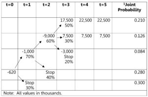
1The joint probability is the probability multiplied along the decision tree, so .7*.6*.5=.210 in the top row, and .7*.60*.3=.126 in the second row, .7*.6*.2=.084 in the third row, .7*.4=.28 in the fourth row, and .3 in the fifth row.
|
2NPV |
3Joint Probability (P) |
NPV x P |
4NPV – E(NPV) |
5P (NPV – E(NPV))2 |
|
34,232.65 |
0.210 |
7,188.86 |
27,771.93 |
161,968,767.54 |
|
6,654.08 |
0.126 |
838.41 |
193.36 |
4,710.78 |
|
-11,324.30 |
0.084 |
-951.24 |
-17,785.02 |
26,569,790.23 |
|
-1,533.24 |
0.280 |
-429.31 |
-7,993.96 |
17,892,961.20 |
|
-620.00 |
0.300 |
-186.00 |
-7,080.72 |
15,040,979.85 |
|
6E(NPV) |
6,460.72 |
Ơ2 |
7221,477,209.61 |
|
|
Ơ |
14,882.11 |
|||
|
CV (Ơ/E(NPV)) |
2.30 |
2This is the NPV of each leg of the decision tree. Starting at the bottom, if the project is abandoned after phase 1, they spent 620,000 so that is the NPV, ie -620. If they continue to phase 2, they spend an additional 1,000,000, so the NPV in the second to the bottom row is -620 – 1,000/(1+.095) = -1,533.24. If they continue to phase 3, they spend another 9,000 and then the path splits 3 ways. Starting at the bottom, they spend an additional 3,000 in year 3, so NPV is -620 – 1,000/(1+.095) – 9,000/(1+.095)^2 – 3,000/(1+.095)^3 = -11,324.30.
3From the decision tree above.
4NPV – E(NPV) is the deviation from the mean and is each NPV minus the expected NPV. For the top row it is 34,232.65-6,460.72=27,771.93.
5This is the 4th column squared (the deviation from the mean squared) times the probability in column 2.
6The expected NPV or E(NPV) is the weighted average of the possible NPVs where the weights are the probabilities of each NPV occurring and is the sum of the NPV X P column.
7This is the sum of the probabilities times the squared deviations from the mean or expected value and is the variance of the Net Present value. See the formula below:
[latex]{\sigma ^2} = \mathop \sum \limits_{i = 1}^n \left[ {{\rho _i}{{\left( {NP{V_i} - E\left( {NPV} \right)} \right)}^2}} \right][/latex]
2. Abandonment: The project could be abandoned at three different points over its life depending on the potential outcomes.
Flexibility: The price could be increased in Years 4 and 5 if demand for the product was high.
Growth: Production could be expanded in Years 4 and 5 if demand for the product was high.
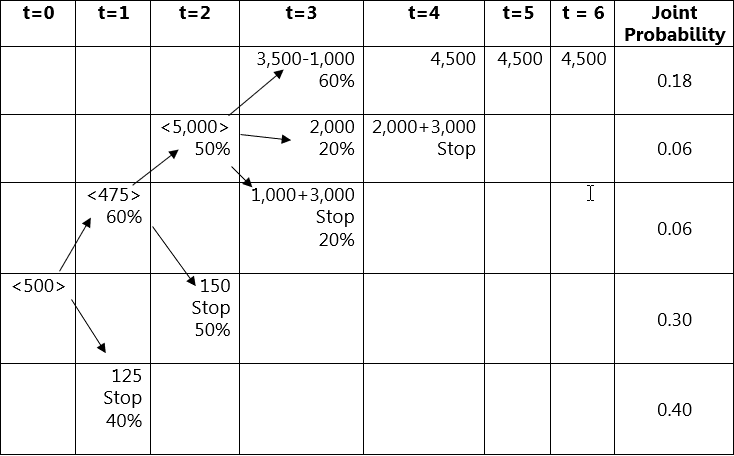
P. Problem: Managing Risk through Management Options at Acme
|
NPV |
Joint Probability (P) |
NPV x P |
NPV – E(NPV) |
P (NPV – E(NPV))2 |
|
4,562.47 |
0.18 |
821.24 |
4,280.25 |
3,297,698.49 |
|
-308.93 |
0.06 |
-18.54 |
-591.14 |
20,966.87 |
|
-2,062.96 |
0.06 |
-123.78 |
-2,345.17 |
329,989.63 |
|
-804.53 |
0.3 |
-241.36 |
-1,086.74 |
354,303.48 |
|
-388.39 |
0.4 |
-155.36 |
-670.61 |
179,886.23 |
|
E(NPV) |
282.22 |
Ơ2 |
4,182,844.70 |
|
|
Ơ |
2,045.20 |
|||
|
CV (Ơ/E(NVP)) |
7.25 |
2. Abandonment: The project could be abandoned at four different points over its life depending on the potential outcomes.
Growth: Production could be expanded to take advantage of high product demand in Years 4, 5, and 6.
Q. Problem: Complex Capital Budgeting with Spreadsheets at Magnum
- See Excel spreadsheet
- See Excel spreadsheet
- Electric cars are the preferred project with a positive NPV and an IRR that exceeds its RRR.
Electric Cars NPV CAD 67,198,203
IRR 24.73% (RRR = 10.00%)
Payback Period 6 Years, 3 Months (15 Year Project)
Solar Generators NPV -CAD 5,325,555
IRR 13.18% (RRR=16.00%)
Payback Period None
NPV of the solar generators project was affected by its high-risk level (more cyclical business in a new industry) and a narrow profit margin. Increasing prices or lowering operating costs should be explored before abandoning the project in order to generate a positive NPV. Also, a larger factory may help the company better meet demand (plant capacity was reached) in the later years of the project which will increase its NPV.
